R Tutorial Series: 2011 ANOVA Article Data

Having wrapped up a recent flurry of R ANOVA articles (and exhausted my knowledge of the subject), I decided to take a look at the R Tutorial Series' Google Analytics data from the past few months.
Since I posted the Two-Way Omnibus ANOVA article on January 17, we have had about 150 visits per day and over 19,000 total page views. The original introduction to R posts are still the most popular ones here, although a few from the regression and ANOVA series are also represented in the most viewed.
I also wanted to share a funny observation about the patterns of visits to the R Tutorial Series. The following graph portrays our daily viewership over the past few months.

The valleys on the chart correspond to the weekends (evidently when no one wants to read about statistical computing). The initial peaks are Mondays, which happen to be when I most often make new posts. Typically, a slightly higher peak comes on Tuesday, followed by a gradual decline back into the weekend valley. Thus, our visits to the R Tutorial Series end up creating a nice little wave pattern throughout the year. The good news with these numbers is that people are reading the R Tutorial Series and (hopefully) learning to use R and apply it to their daily work, which is the blog's ultimate purpose. I also appreciate all of the comments, questions, and tips that have been posted by readers. Your feedback really helps to improve the tutorials.

Upcoming Plans

As mentioned, I have concluded my planned coverage of ANOVA in R. Thus, we have reached a sort of break period, much like the one that followed last year's spurt of regression tutorials. I do plan to keep writing R tutorials, but for the time being, they may arrive in less predictable intervals and cover a wider variety of content. As always, I welcome contact regarding guest posts, especially on statistical and R content that I have not covered or am not yet familiar with.

R Tutorial Series: Applying the Reshape Package to Organize ANOVA Data

As demonstrated in the preceding ANOVA tutorials, data organization is central to conducting ANOVA in R. In standard ANOVA, we used the tapply() function to generate a table for a single summary function. In repeated measures ANOVA, we used separate datasets for our omnibus ANOVA and follow-up comparisons. This tutorial will demonstrate how the reshape package can be used to simplify the ANOVA data organization process in R.

Tutorial Files

Before we begin, you may want to download the between group and repeated measures datasets (.csv) used in this tutorial. Be sure to right-click and save the files to your R working directory. The between groups dataset contains a hypothetical sample of 30 cases separated into three groups (a, b, and c). The repeated measures dataset contains a hypothetical sample of 10 cases across three measurements (a, b, and c). In both cases, the values are represented on a scale that ranges from 1 to 5.

Beginning Steps

To begin, we need to read our datasets into R and store their contents in variables.

1. > #read the datasets into R variables using the read.csv(file) function
2. > dataBetween <- read.csv("dataset_ANOVA_reshape_1.csv")
3. > dataRepeated <- read.csv("dataset_ANOVA_reshape_2.csv")

Reshape Package

Next, we need to install and load the reshape package. In this tutorial, we will make use of the package's cast() and melt() functions.

1. > #install the package
2. > install.packages("reshape")
3. > #load the package
4. > library(reshape)

Using cast() to Derive ANOVA Descriptives

The cast() function can be used to easily derive summary statistics for a between groups ANOVA dataset. The cast() function receives the following primary arguments.

• data: the dataset
• formula: in our case, a one-sided formula indicating the grouping variable
• fun.aggregate: a function or vector of functions for deriving summary statistics, such as mean, var, or sd

1. > #display the raw between groups data
2. > dataBetween

The raw between groups data

1. > #cast the between groups data using cast(data, formula, fun.aggregate) to get the group means
2. > cast(dataBetween, formula = ~group, fun.aggregate = mean)

The casted data with means

Note that the fun.aggregate argument can also receive a vector of summary statistics functions. This will yield all of the requested descriptives via a single cast() function.

1. > #cast the between groups data using cast(data, formula, fun.aggregate) to get the group means, variances, and standard deviations
2. > cast(dataBetween, formula = ~group, fun.aggregate = c(mean, var, sd))

The casted data with descriptives

Using melt() to Prepare Repeated Measures Data for Pairwise Comparisons

The melt() function can be used to morph a repeated measures ANOVA dataset prior to conducting pairwise comparisons. The melt() function receives the following primary arguments.

• data: the dataset
• id.vars: the id variable or a vector of values that can be used as ids
• measure.vars: a vector containing the variables to be melted
• variable_name: the name of the column containing the melted variables

1. > #display the repeated measures data
2. > dataRepeated

The raw repeated measures data

1. > #melt the repeated measures data using melt(data, id.vars, measure.vars, variable_name) to organize it for pairwise comparisons
2. > melt(dataRepeated, id.vars = "case", measure.vars = c("valueA", "valueB", "valueC"), variable_name = "abcValues")

The melted repeated measures data

Note that the data are now prepared to be used in the pairwise.t.test() function. See the One-Way ANOVA with Pairwise Comparisons tutorial for details on using the pairwise.t.test() function.

Complete ANOVA Reshape Example

To see a complete example of how ANOVA data can be organized using the reshape package in R, please download the ANOVA reshape example (.txt) file.

R Tutorial Series: ANOVA Pairwise Comparison Methods

When we have a statistically significant effect in ANOVA and an independent variable of more than two levels, we typically want to make follow-up comparisons. There are numerous methods for making pairwise comparisons and this tutorial will demonstrate how to execute several different techniques in R.

Tutorial Files

Before we begin, you may want to download the sample data (.csv) used in this tutorial. Be sure to right-click and save the file to your R working directory. This dataset contains a hypothetical sample of 30 participants who are divided into three stress reduction treatment groups (mental, physical, and medical). The values are represented on a scale that ranges from 1 to 5. This dataset can be conceptualized as a comparison between three stress treatment programs, one using mental methods, one using physical training, and one using medication. The values represent how effective the treatment programs were at reducing participant's stress levels, with higher numbers indicating higher effectiveness.

Beginning Steps

To begin, we need to read our dataset into R and store its contents in a variable.

1. > #read the dataset into an R variable using the read.csv(file) function
2. > dataPairwiseComparisons <- read.csv("dataset_ANOVA_OneWayComparisons.csv")
3. > #display the data
4. > dataPairwiseComparisons

The first ten rows of our dataset

Omnibus ANOVA

For the purposes of this tutorial, we will assume that the omnibus ANOVA has already been conducted and that the main effect for treatment was statistically significant. For details on this process, see the One-Way ANOVA with Pairwise Comparisons tutorial, which uses the same dataset.

Means

Let's also look at the means of our treatment groups. Here, we will use the tapply() function, along with the following arguments, to generate a table of means.

• X: the data
• INDEX: a list() of factor variables
• FUN: the function to be applied

1. > #use tapply(X, INDEX, FUN) to generate a table displaying each treatment group mean
2. > tapply(X = dataPairwiseComparisons$StressReduction, INDEX = list(dataPairwiseComparisons$Treatment), FUN = mean)

The treatment group means

Pairwise Comparisons

We will cover five major techniques for controlling Type I error when making pairwise comparisons. These methods are no adjustment, Bonferroni's adjustment, Holm's adjustment, Fisher's LSD, and Tukey's HSD. All of these techniques will be demonstrated on our sample dataset, although the decision as to which to use in a given situation is left up to the reader.

pairwise.t.test()

Our first three methods will make use of the pairwise.t.test() function, which has the following major arguments.

• x: the dependent variable
• g: the independent variable
• p.adj: the p-value adjustment method used to control for the family-wise Type I error rate across the comparisons; one of "none", "bonferroni", "holm", "hochberg", "hommel", "BH", or "BY"

No Adjustment

Using p.adj = "none" in the pairwise.t.test() function makes no correction for the Type I error rate across the pairwise tests. This technique can be useful for employing methods that are not already built into R functions, such as the Shaffer/Modified Shaffer, which use different alpha level divisors based on the number of levels composing the independent variable. The console results will contain no adjustment, but the researcher can manually consider the statistical significance of the p-values under his or her desired alpha level.

1. > #use pairwise.t.test(x, g, p.adj) to test the pairwise comparisons between the treatment group means
2. > #no adjustment
3. > pairwise.t.test(dataPairwiseComparisons$StressReduction, dataPairwiseComparisons$Treatment, p.adj = "none")

Pairwise comparisons of treatment group means with no adjustment

With no adjustment, the mental-medical and physical-medical comparisons are statistically significant, whereas the mental-physical comparison is not. This suggests that both the mental and physical treatments are superior to the medical treatment, but that there is insufficient statistical support to distinguish between the mental and physical treatments.

Bonferroni Adjustment

The Bonferroni adjustment simply divides the Type I error rate (.05) by the number of tests (in this case, three). Hence, this method is often considered overly conservative. The Bonferroni adjustment can be made using p.adj = "bonferroni" in the pairwise.t.test() function.

1. > #Bonferroni adjustment
2. > pairwise.t.test(dataPairwiseComparisons$StressReduction, dataPairwiseComparisons$Treatment, p.adj = "bonferroni")

Pairwise comparisons of treatment group means using Bonferroni adjustment

Using the Bonferroni adjustment, only the mental-medical comparison is statistically significant. This suggests that the mental treatment is superior to the medical treatment, but that there is insufficient statistical support to distinguish between the mental and physical treatments and the physical and medical treatments. Notice that these results are more conservative than with no adjustment.

Holm Adjustment

The Holm adjustment sequentially compares the lowest p-value with a Type I error rate that is reduced for each consecutive test. In our case, this means that our first p-value is tested at the .05/3 level (.017), second at the .05/2 level (.025), and third at the .05/1 level (.05). This method is generally considered superior to the Bonferroni adjustment and can be employed using p.adj = "holm" in the pairwise.t.test() function.

1. > #Holm adjustment
2. > pairwise.t.test(dataPairwiseComparisons$StressReduction, dataPairwiseComparisons$Treatment, p.adj = "holm")

Pairwise comparisons of treatment group means using Holm adjustment

Using the Holm procedure, our results are practically (but not mathematically) identical to using no adjustment.

LSD Method

The Fisher Least Significant Difference (LSD) method essentially does not correct for the Type I error rate for multiple comparisons and is generally not recommended relative to other options. However, should the need arise to employ this method, one should seek out the LSD.test() function in the agricolae package, which has the following major arguments.

• y: the dependent variable
• trt: the independent variable
• DFerror: the degrees of freedom error
• MSerror: the mean squared error

Note that the DFerror and MSerror can be found in the omnibus ANOVA table.

1. > #load the agricolae package (install first, if necessary)
2. > library(agricolae)
3. #LSD method
4. #use LSD.test(y, trt, DFerror, MSerror) to test the pairwise comparisons between the treatment group means
5. > LSD.test(dataPairwiseComparisons$StressReduction, dataPairwiseComparisons$Treatment, 30.5, 1.13)

Pairwise comparisons of treatment group means using LSD method

Using the LSD method, our results are practically (but not mathematically) identical to using no adjustment or the Holm procedure.

HSD Method

The Tukey Honest Significant Difference (HSD) method controls for the Type I error rate across multiple comparisons and is generally considered an acceptable technique. This method can be executed using the TukeyHSD(x) function, where x is a linear model object created using the aov(formula, data) function. Note that in this application, the aov(formula, data) function is identical to the lm(formula, data) that we are already familiar with from linear regression.

1. > #HSD method
2. > #use TukeyHSD(x), in tandem with aov(formula, data), to test the pairwise comparisons between the treatment group means
3. TukeyHSD(aov(StressReduction ~ Treatment, dataPairwiseComparisons))

Pairwise comparisons of treatment group means using HSD method

Using the HSD method, our results are practically (but not mathematically) identical to using the Bonferroni, Holm, or LSD methods.

Complete Pairwise Comparisons Example

To see a complete example of how various pairwise comparison techniques can be applied in R, please download the ANOVA pairwise comparisons example (.txt) file.

R Tutorial Series: Two-Way ANOVA with Unequal Sample Sizes

When the sample sizes within the levels of our independent variables are not equal, we have to handle our ANOVA differently than in the typical two-way case. This tutorial will demonstrate how to conduct a two-way ANOVA in R when the sample sizes within each level of the independent variables are not the same.

Tutorial Files

Before we begin, you may want to download the sample data (.csv) used in this tutorial. Be sure to right-click and save the file to your R working directory. This dataset contains a hypothetical sample of 30 students who were exposed to one of two learning environments (offline or online) and one of two methods of instruction (classroom or tutor), then tested on a math assessment. Possible math scores range from 0 to 100 and indicate how well each student performed on the math assessment. Each student participated in either an offline or online learning environment and received either classroom instruction (i.e. one to many) or instruction from a personal tutor (i.e. one to one).

Beginning Steps

To begin, we need to read our dataset into R and store its contents in a variable.

1. > #read the dataset into an R variable using the read.csv(file) function
2. > dataTwoWayUnequalSample <- read.csv("dataset_ANOVA_TwoWayUnequalSample.csv")
3. > #display the data
4. > dataTwoWayUnequalSample

The first ten rows of our dataset

Unequal Sample Sizes

In our study, 16 students participated in the online environment, whereas only 14 participated in the offline environment. Further, 20 students received classroom instruction, whereas only 10 received personal tutor instruction. As such, we should take action to compensate for the unequal sample sizes in order to retain the validity of our analysis. Generally, this comes down to examining the correlation between the factors and the causes of the unequal sample sizes en route to choosing whether to use weighted or unweighted means - a decision which can drastically impact the results of an ANOVA. This tutorial will demonstrate how to conduct ANOVA using both weighted and unweighted means. Thus, the ultimate decision as to the use of weighted or unweighted means is left up to each individual and his or her specific circumstances.

Weighted Means

First, let's suppose that we decided to go with weighted means, which take into account the correlation between our factors that results from having treatment groups with different sample sizes. A weighted mean is calculated by simply adding up all of the values and dividing by the total number of values. Consequently, we can easily derive the weighted means for each treatment group using our subset(data, condition) and mean(data) functions.

1. > #use subset(data, condition) to create subsets for each treatment group
2. > #offline subset
3. > offlineData <- subset(dataTwoWayUnequalSample, dataTwoWayUnequalSample$environment == "offline")
4. > #online subset
5. > onlineData <- subset(dataTwoWayUnequalSample, dataTwoWayUnequalSample$environment == "online")
6. > #classroom subset
7. > classroomData <- subset(dataTwoWayUnequalSample, dataTwoWayUnequalSample$instruction == "classroom")
8. > #tutor subset
9. > tutorData <- subset(dataTwoWayUnequalSample, dataTwoWayUnequalSample$instruction == "tutor")
10. > #use mean(data) to calculate the weighted means for each treatment group
11. > #offline weighted mean
12. > mean(offlineData$math)
13. > #online weighted mean
14. > mean(onlineData$math)
15. > #classroom weighted mean
16. > mean(classroomData$math)
17. > #tutor weighted mean
18. > mean(tutorData$math)

The weighted means for the environment and instruction conditions

ANOVA using Type I Sums of Squares

When applying weighted means, it is suggested that we use Type I sums of squares (SS) in our ANOVA. Type I happens to be the default SS used in our standard anova(object) function, which will be used to execute our analysis. Note that in the case of two-way ANOVA, the ordering of our independent variables matters when using weighted means. Therefore, we must run our ANOVA two times, once with each independent variable taking the lead. However, the interaction effect is not affected by the ordering of the independent variables.

1. > #use anova(object) to execute the Type I SS ANOVAs
2. > #environment ANOVA
3. > anova(lm(math ~ environment * instruction, dataTwoWayUnequalSample))
4. > #instruction ANOVA
5. > anova(lm(math ~ instruction * environment, dataTwoWayUnequalSample))

The Type I SS ANOVA results. Note the differences in main effects based on the ordering of the independent variables.

These results indicate statistically insignificant main effects for both the environment and instruction variables, as well as the interaction between them.

Unweighted Means

Now let's turn to using unweighted means, which essentially ignore the correlation between the independent variables that arise from unequal sample sizes. An unweighted mean is calculated by taking the average of the individual group means. Thus, we can derive our unweighted means by summing the means of each level of our independent variables and dividing by the total number of levels. For instance, to find the unweighted mean for environment, we will add the means for our offline and online groups, then divide by two.

1. > #use mean(data) and subset(data, condition) to calculate the unweighted means for each treatment group
2. > #offline unweighted mean = (classroom offline mean + tutor offline mean) / 2
3. (mean(subset(offlineData$math, offlineData$instruction == "classroom")) + mean(subset(offlineData$math, offlineData$instruction == "tutor"))) / 2
4. > #online unweighted mean = (classroom online mean + tutor online mean) / 2
5. > (mean(subset(onlineData$math, onlineData$instruction == "classroom")) + mean(subset(onlineData$math, onlineData$instruction == "tutor"))) / 2
6. > #classroom unweighted mean = (offline classroom mean + online classroom mean) / 2
7. > (mean(subset(classroomData$math, classroomData$environment == "offline")) + mean(subset(classroomData$math, classroomData$environment == "online"))) / 2
8. > #tutor unweighted mean = (offline tutor mean + online tutor mean) / 2
9. > (mean(subset(tutorData$math, tutorData$environment == "offline")) + mean(subset(tutorData$math, tutorData$environment == "online"))) / 2

The unweighted means for the environment and instruction conditions

ANOVA using Type III Sums of Squares

When applying unweighted means, it is suggested that we use Type III sums of squares (SS) in our ANOVA. Type III SS can be set using the type argument in the Anova(mod, type) function, which is a member of the car package.

1. > #load the car package (install first, if necessary)
2. > library(car)
3. > #use the Anova(mod, type) function to conduct the Type III SS ANOVA
4. > Anova(lm(math ~ environment * instruction, dataTwoWayUnequalSample), type = "3")

The Type III SS ANOVA results.

Once again, our ANOVA results indicate statistically insignificant main effects for both the environment and instruction variables, as well as the interaction between them. However, it is worth noting that both the means and p-values are different when using unweighted means and Type III SS compared to weighted means and Type I SS. In certain cases, this difference can be quite pronounced and lead to entirely different outcomes between the two methods. Hence, choosing the appropriate means and SS for a given analysis is a matter that should be approached with conscious consideration.

Pairwise Comparisons

Note that since our independent variables contain only two levels, there is no need to conduct follow-up comparisons. However, should you reach this point with a statistically significant independent variable of more than three levels, you could conduct pairwise comparisons in the same manner as demonstrated in the Two-Way ANOVA with Comparisons tutorial.

Complete Two-Way ANOVA with Unequal Sample Sizes Example

To see a complete example of how two-way ANOVA with unequal sample sizes can be conducted in R, please download the two-way ANOVA with unequal sample sizes example (.txt) file.

R Tutorial Series: Two-Way Repeated Measures ANOVA

Repeated measures data require a different analysis procedure than our typical two-way ANOVA and subsequently follow a different R process. This tutorial will demonstrate how to conduct two-way repeated measures ANOVA in R using the Anova() function from the car package.
Note that the two-way repeated measures ANOVA process can be very complex to organize and execute in R. Although it has been distilled into just a few small steps in this guide, it is recommended that you fully and precisely complete the example before experimenting with your own data. As you will see, organization of the raw data is critical to successfully conducting a two-way repeated measures ANOVA using the demonstrated technique.

Tutorial Files

Before we begin, you may want to download the sample data (.csv) and sample idata frame (.csv) used in this tutorial. Be sure to right-click and save the files to your R working directory. This dataset contains a hypothetical sample of 30 participants whose interest in school and interest in work was measured at three different ages (10, 15, and 20). The interest values are represented on a scale that ranges from 1 to 5 and indicate how interested each participant was in a given topic at each given age.

Data Setup

Notice that our data are arranged differently for a repeated measures ANOVA. In a typical two-way ANOVA, we would place all of the values of our independent variable in a single column and identify their respective levels with a second column, as demonstrated in this sample two-way dataset. In a two-way repeated measures ANOVA, we instead combine each independent variable with its time interval, thus yielding columns for each pairing. Hence, rather than having one vertical column for school interest and one for work interest, with a second column for age, we have six separate columns for interest, three for school interest and three for work interest at each age level. The following graphic is intended to help demonstrate this organization method.

Treat time as if it were an independent variable. Then combine each independent variable with each level of time and arrange the columns horizontally.

Beginning Steps

To begin, we need to read our dataset into R and store its contents in a variable.

1. > #read the dataset into an R variable using the read.csv(file) function
2. > dataTwoWayRepeatedMeasures <- read.csv("dataset_ANOVA_TwoWayRepeatedMeasures.csv")
3. > #display the data
4. > #notice the atypical column arrangement for repeated measures data
5. > dataTwoWayRepeatedMeasures

The first ten rows of our dataset

idata Frame

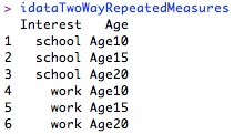
Another item that we need to import for this analysis is our idata frame. This object will be used in our Anova() function to define the structure of our analysis.

1. > #read the idata frame into an R variable
2. > idataTwoWayRepeatedMeasures <- read.csv("idata_ANOVA_TwoWayRepeatedMeasures.csv")
3. > #display the idata frame
4. > #notice the text values and correspondence between our idata rows and the columns in our dataset
5. > idataTwoWayRepeatedMeasures

The idata frame

Note that it is critical that your idata frame take the demonstrated form for this technique to work. I experimented with several alternative, perhaps more intuitive, layouts without success. It is particularly important to notice that both columns of the idata frame contain text values (not numerical ones - hence the repeated prefixing of Age to the values in every row of the Age column). Additionally, if you read the rows of the idata frame horizontally, you will see that they correspond precisely to the columns of our dataset. The following graphic is intended to help demonstrate this organization method.

Use only text values in your idata frame. Ensure that the rows of your idata frame correspond to the columns in your dataset.

Linear Model

Prior to executing our analysis, we must follow two steps to formulate our linear model to be used in the Anova() function.

Step 1: Bind the Columns

1. > #use cbind() to bind the columns of the original dataset
2. > interestBind <- cbind(dataTwoWayRepeatedMeasures$schoolAge10, dataTwoWayRepeatedMeasures$schoolAge15, dataTwoWayRepeatedMeasures$schoolAge20, dataTwoWayRepeatedMeasures$workAge10, dataTwoWayRepeatedMeasures$workAge15, dataTwoWayRepeatedMeasures$workAge20)

Step 2: Define the Model

1. > #use lm() to generate a linear model using the bound columns from step 1
2. > interestModel <- lm(interestBind ~ 1)

Anova(mod, idata, idesign) Function

Typically, researchers will choose one of several techniques for analyzing repeated measures data, such as an epsilon-correction method, like Huynh-Feldt or Greenhouse-Geisser, or a multivariate method, like Wilks' Lambda or Hotelling's Trace. Conveniently, having already prepared our data, we can employ a single Anova(mod, idata, idesign) function from the car package to yield all of the relevant repeated measures results. This allows us simplicity in that only a single function is required, regardless of the technique that we wish to employ. Thus, witnessing our outcomes becomes as simple as locating the desired method in the cleanly printed results.
Our Anova(mod, idata, idesign) function will be composed of three arguments. First, mod will contain our linear model. Second, idata will contain our data frame. Third, idesign will contain a multiplication of the row headings from our idata frame (in other words, our independent variables), preceded by a tilde (~). Thus, our final function takes on the following form.

1. > #load the car package (install first, if necessary)
2. library(car)
3. > #compose the Anova(mod, idata, idesign) function
4. > analysis <- Anova(interestModel, idata = idataTwoWayRepeatedMeasures, idesign = ~Interest * Age)

Results Summary

Finally, we can use the summary(object) function to visualize the results of our repeated measures ANOVA.

1. > #use summary(object) to visualize the results of the repeated measures ANOVA
2. > summary(analysis)

Relevant segment of repeated measures ANOVA results

Supposing that we are interested in the Wilks' Lambda method, we can see that there is a statistically significant interaction effect between interest in school and interest in work across the age groups (p < .001). This suggests that we should further examine our data at the level of simple main effects. For more information investigating on simple main effects, see the Two-Way ANOVA with Interactions and Simple Main Effects tutorial. Of course, in this case of repeated measures ANOVA, another way to break the data down would be to run two one-way repeated measures ANOVAs, one for each of the independent variables. In either instance, pairwise comparisons can be conducted to determine the significance of the differences between the levels of any significant effects.

Complete Two-Way Repeated Measures ANOVA Example

To see a complete example of how two-way repeated measures ANOVA can be conducted in R, please download the two-way repeated measures ANOVA example (.txt) file.

References

Moore, Colleen. (n.d.). 610 R9 -- Two-way Repeated-measures Anova. Retrieved January 21, 2011 from http://psych.wisc.edu/moore/Rpdf/610-R9_Within2way.pdf

R Tutorial Series: One-Way Repeated Measures ANOVA

Repeated measures data require a different analysis procedure than our typical one-way ANOVA and subsequently follow a different R process. This tutorial will demonstrate how to conduct one-way repeated measures ANOVA in R using the Anova(mod, idata, idesign) function from the car package.

Tutorial Files

Before we begin, you may want to download the sample data (.csv) used in this tutorial. Be sure to right-click and save the file to your R working directory. This dataset contains a hypothetical sample of 30 participants whose interest in voting was measured at three different ages (10, 15, and 20). The interest values are represented on a scale that ranges from 1 to 5 and indicate how interested each participant was in voting at each given age.

Data Setup

Notice that our data are arranged differently for a repeated measures ANOVA. In a typical one-way ANOVA, we would place all of the values of our independent variable in a single column and identify their respective levels with a second column, as demonstrated in this sample one-way dataset. In a repeated measures ANOVA, we instead treat each level of our independent variable as if it were a variable, thus placing them side by side as columns. Hence, rather than having one vertical column for voting interest, with a second column for age, we have three separate columns for voting interest, one for each age level.

Beginning Steps

To begin, we need to read our dataset into R and store its contents in a variable.

1. > #read the dataset into an R variable using the read.csv(file) function
2. > dataOneWayRepeatedMeasures <- read.csv("dataset_ANOVA_OneWayRepeatedMeasures.csv")
3. > #display the data
4. > #notice the atypical column arrangement for repeated measures data
5. > dataOneWayRepeatedMeasures

The first ten rows of our dataset

Preparing the Repeated Measures Factor

Prior to executing our analysis, we must follow a small series of steps in order to prepare our repeated measures factor.

Step 1: Define the Levels

1. > #use c() to create a vector containing the number of levels within the repeated measures factor
2. > #create a vector numbering the levels for our three voting interest age groups
3. > ageLevels <- c(1, 2, 3)

Step 2: Define the Factor

1. > #use as.factor() to create a factor using the level vector from step 1
2. > #convert the age levels into a factor
3. > ageFactor <- as.factor(ageLevels)

Step 3: Define the Frame

1. > #use data.frame() to create a data frame using the factor from step 2
2. > #convert the age factor into a data frame
3. > ageFrame <- data.frame(ageFactor)

Step 4: Bind the Columns

1. > #use cbind() to bind the levels of the factor from the original dataset
2. > #bind the age columns
3. > ageBind <- cbind(dataOneWayRepeatedMeasures$Interest10, dataOneWayRepeatedMeasures$Interest15, dataOneWayRepeatedMeasures$Interest20)

Step 5: Define the Model

1. > #use lm() to generate a linear model using the bound factor levels from step 4
2. > #generate a linear model using the bound age levels
3. > ageModel <- lm(ageBind ~ 1)

Employing the Anova(mod, idata, idesign) Function

Typically, researchers will choose one of several techniques for analyzing repeated measures data, such as an epsilon-correction method, like Huynh-Feldt or Greenhouse-Geisser, or a multivariate method, like Wilks' Lambda or Hotelling's Trace. Conveniently, having already prepared our data, we can employ a single Anova(mod, idata, idesign) function from the car package to yield all of the relevant repeated measures results. This allows us simplicity in that only a single function is required, regardless of the technique that we wish to employ. Thus, witnessing our outcomes becomes as simple as locating the desired method in the cleanly printed results.
Our Anova(mod, idata, idesign) function will be composed of three arguments. First, mod will contain our linear model from Step 5 in the preceding section. Second, idata will contain our data frame from Step 3. Third, idesign will contain our factor from Step 2, preceded by a tilde (~). Thus, our final function takes on the following form.

1. > #load the car package (install first, if necessary)
2. library(car)
3. > #compose the Anova(mod, idata, idesign) function
4. > analysis <- Anova(ageModel, idata = ageFrame, idesign = ~ageFactor)

Visualizing the Results

Finally, we can use the summary(object) function to visualize the results of our repeated measures ANOVA.

1. > #use summary(object) to visualize the results of the repeated measures ANOVA
2. > summary(analysis)

Relevant segment of repeated measures ANOVA results

Supposing that we are interested in the Wilks' Lambda method, we can see that the differences in the means for voting interest at ages 10, 15, and 20 are statistically significant (p < .001).

Pairwise Comparisons

Note that we could conduct follow-up comparisons on our age factor to determine which age level means are significantly different from one another. For this purpose, it is recommended that the data be rearranged into the standard ANOVA format that we have used throughout our other tutorials. Subsequently, we could conduct pairwise comparisons in the same manner as demonstrated in the One-Way ANOVA with Comparisons tutorial.

Complete One-Way Repeated Measures ANOVA Example

To see a complete example of how one-way repeated measures ANOVA can be conducted in R, please download the one-way repeated measures ANOVA example (.txt) file.

R Tutorial Series: Two-Way ANOVA with Interactions and Simple Main Effects

When an interaction is present in a two-way ANOVA, we typically choose to ignore the main effects and elect to investigate the simple main effects when making pairwise comparisons. This tutorial will demonstrate how to conduct pairwise comparisons when an interaction is present in a two-way ANOVA.

Tutorial Files

Before we begin, you may want to download the sample data (.csv) used in this tutorial. Be sure to right-click and save the file to your R working directory. This dataset contains a hypothetical sample of 60 participants who are divided into three stress reduction treatment groups (mental, physical, and medical) and two gender groups (male and female). The stress reduction values are represented on a scale that ranges from 1 to 5. This dataset can be conceptualized as a comparison between three stress treatment programs, one using mental methods, one using physical training, and one using medication across genders. The values represent how effective the treatment programs were at reducing participant's stress levels, with higher numbers indicating higher effectiveness.

Beginning Steps

To begin, we need to read our dataset into R and store its contents in a variable.

1. > #read the dataset into an R variable using the read.csv(file) function
2. > dataTwoWayInteraction <- read.csv("dataset_ANOVA_TwoWayInteraction.csv")
3. > #display the data
4. > dataTwoWayInteraction

The first ten rows of our dataset.

Omnibus Test

Let's run a general omnibus test to assess the main effects and interactions present in the dataset.

1. > #use anova(object) to test the omnibus hypothesis
2. > #Are main effects or interaction effects present in the independent variables?
3. > anova(lm(StressReduction ~ Treatment * Gender, dataTwoWayInteraction))

The omnibus ANOVA test

Divide the Data

The significant omnibus interaction suggests that we should ignore the main effects and instead investigate the simple main effects for our independent variables. To do so, we need to divide our dataset along each level of our treatment variable. We can create subsets of our dataset using the subset(data, condition) function, where data is the original dataset and condition contains the parameters defining the subset.

1. > #use subset(data, condition) to divide the original dataset
2. > #medical subset
3. > dataMedical <- subset(dataTwoWayInteraction, Treatment == "medical")
4. > #mental subset
5. > dataMental <- subset(dataTwoWayInteraction, Treatment == "mental")
6. > #physical subset
7. > dataPhysical <- subset(dataTwoWayInteraction, Treatment == "physical")

Group ANOVAs

With datasets representing each of our treatment groups, we can now run an ANOVA for each that investigates the impact of gender. You may notice that this is effectively running three one-way ANOVAs with gender being the independent variable. Therefore, we should control for Type I error by dividing our typical .05 alpha level by three (.017).

1. > #run ANOVA on the treatment subsets to investigate the impacts of gender within each
2. > #medical
3. > anova(lm(StressReduction ~ Gender, dataMedical))
4. > #mental
5. > anova(lm(StressReduction ~ Gender, dataMental))
6. > #physical
7. > anova(lm(StressReduction ~ Gender, dataPhysical))

The gender within treatment group ANOVA tests

At an alpha level of .017, the gender effect within the mental (p = .014) and physical (p < .001) groups was statistically significant. In the mental condition, the means are 3 for males and 4 for females. In the physical condition, the means are 4 for males and 2 for females. These results suggest that the mental treatment is more effective in reducing stress for females than males, while the physical treatment is more effective for males than females. Further, there is insufficient statistical support for a gender difference in the medical treatment.

Pairwise Comparisons

Note that since our gender variable contains only two levels, there is no need to conduct follow-up comparisons. However, should you reach this point with an independent variable of more than three levels, you could conduct pairwise comparisons in the same manner as demonstrated in the Two-Way ANOVA with Comparisons tutorial. In this case, remember to carry through your reduced Type I error rate from the preceding ANOVA tests.

Complete Two-Way ANOVA with Interactions Example

To see a complete example of how two-way ANOVA simple main effects can be explored in R, please download the two-way ANOVA interaction example (.txt) file.

R Tutorial Series: Two-Way ANOVA with Pairwise Comparisons

By extending our one-way ANOVA procedure, we can test the pairwise comparisons between the levels of several independent variables. This tutorial will demonstrate how to conduct pairwise comparisons in a two-way ANOVA.

Tutorial Files

Before we begin, you may want to download the sample data (.csv) used in this tutorial. Be sure to right-click and save the file to your R working directory. This dataset contains a hypothetical sample of 27 participants who are divided into three stress reduction treatment groups (mental, physical, and medical) and three age groups (young, mid, and old). The stress reduction values are represented on a scale that ranges from 0 to 10. This dataset can be conceptualized as a comparison between three stress treatment programs, one using mental methods, one using physical training, and one using medication, across three age groups. The stress reduction values represent how effective the treatment programs were at reducing participant's stress levels, with higher numbers indicating higher effectiveness. Note that the numbers in this dataset are not very realistic and are simply used to make this example possible.

Beginning Steps

To begin, we need to read our dataset into R and store its contents in a variable.

1. > #read the dataset into an R variable using the read.csv(file) function
2. > dataTwoWayComparisons <- read.csv("dataset_ANOVA_TwoWayComparisons.csv")
3. > #display the data
4. > dataTwoWayComparisons

The first ten rows of our dataset.

Omnibus Test

Let's run a general omnibus test to assess the main effects and interactions present in the dataset.

1. > #use anova(object) to test the omnibus hypothesis
2. > #Are main effects or interaction effects present in the independent variables?
3. > anova(lm(StressReduction ~ Treatment * Age, dataTwoWayComparisons))

The omnibus ANOVA test

Pairwise Comparisons

Since the omnibus test was significant for both variables and no interaction effect was present, we can proceed to testing the main effect pairwise comparisons. To accomplish this, we will apply our pairwise.t.test() function to each of our independent variables. For more details on the pairwise.t.test() function, see the One-Way ANOVA with Pairwise Comparisons tutorial.

1. > #use pairwise.t.test(x, g, p.adj) to test the pairwise comparisons between the treatment group means
2. > #What significant differences are present amongst the treatment means?
3. > pairwise.t.test(dataTwoWayComparisons$StressReduction, dataTwoWayComparisons$Treatment, p.adj = "none")
4. > #use pairwise.t.test(x, g, p.adj) to test the pairwise comparisons between the age group means
5. > #What significant differences are present amongst the age group means?
6. > pairwise.t.test(dataTwoWayComparisons$StressReduction, dataTwoWayComparisons$Age, p.adj = "none")

Pairwise comparisons of treatment group means

Pairwise comparisons of age group means

Note that the desired p-adjustment method will vary by researcher, study, etc. Here, we will assume an alpha level of .05 for all tests, effectively making no adjustment for the family-wise Type I error rate.
These results indicate that there are are no statistically significant pairwise differences between the treatment groups and that all of the comparisons between age groups are statistically significant. The age group means are 8 for young, 5 for mid, and 2 for old. Consequently, we are inclined to conclude that, regardless of treatment, young patients are going to be most responsive, followed by middle aged patients, followed by older ones. However, there is insufficient support to differentiate between the effectiveness of the treatment methods themselves.

Complete Two-Way ANOVA with Pairwise Comparisons Example

To see a complete example of how two-way ANOVA pairwise comparisons can be conducted in R, please download the two-way ANOVA comparisons example (.txt) file.

R Tutorial Series: One-Way ANOVA with Pairwise Comparisons

When we have more than two groups in a one-way ANOVA, we typically want to statistically assess the differences between each group. Whereas a one-way omnibus ANOVA assesses whether a significant difference exists at all amongst the groups, pairwise comparisons can be used to determine which group differences are statistically significant.

Tutorial Files

Before we begin, you may want to download the sample data (.csv) used in this tutorial. Be sure to right-click and save the file to your R working directory. This dataset contains a hypothetical sample of 30 participants who are divided into three stress reduction treatment groups (mental, physical, and medical). The values are represented on a scale that ranges from 1 to 5. This dataset can be conceptualized as a comparison between three stress treatment programs, one using mental methods, one using physical training, and one using medication. The values represent how effective the treatment programs were at reducing participant's stress levels, with higher numbers indicating higher effectiveness.

Beginning Steps

To begin, we need to read our dataset into R and store its contents in a variable.

1. > #read the dataset into an R variable using the read.csv(file) function
2. > dataOneWayComparisons <- read.csv("dataset_ANOVA_OneWayComparisons.csv")
3. > #display the data
4. > dataOneWayComparisons

The first ten rows of our dataset.

Omnibus Test

One way to begin an ANOVA is to run a general omnibus test. The advantage to starting here is that if the omnibus test comes up insignificant, you can stop your analysis and deem all pairwise comparisons insignificant. If the omnibus test is significant, you should continue with pairwise comparisons.

1. > #use anova(object) to test the omnibus hypothesis
2. > #Is there a significant difference amongst the treatment means?
3. > anova(lm(StressReduction ~ Treatment, dataOneWayComparisons))

The omnibus ANOVA test

Pairwise Comparisons

Since the omnibus test was significant, we are safe to continue with our pairwise comparisons. To make pairwise comparisons between the treatment groups, we will use the pairwise.t.test() function, which has the following major arguments.

• x: the dependent variable
• g: the independent variable
• p.adj: the p-value adjustment method used to control for the family-wise Type I error rate across the comparisons; one of "none", "bonferroni", "holm", "hochberg", "hommel", "BH", or "BY"

The pairwise.t.test() function can be implemented as follows.

1. > #use pairwise.t.test(x, g, p.adj) to test the pairwise comparisons between the treatment group means
2. > #What significant differences are present amongst the treatment means?
3. > pairwise.t.test(dataOneWayComparisons$StressReduction, dataOneWayComparisons$Treatment, p.adj = "none")

Pairwise comparisons of treatment group means

Note that the desired p-adjustment method will vary by researcher, study, etc. Here, we will assume an alpha level of .05 for all tests, effectively making no adjustment for the family-wise Type I error rate.
These results indicate that there is a statistically significant difference between the mental and medical (p = .004) and physical and medical (p = 0.045), but not the mental and physical (p = 0.302) treatments. The treatment means are 3.5 for mental, 3 for physical, and 2 for medical. Subsequently, we are inclined to conclude based on this study that the mental and physical treatments lead to greater stress reduction than the medical method, but that there is insufficient statistical support to determine that either the mental or physical treatment method is superior.

Complete One-Way ANOVA with Pairwise Comparisons Example

To see a complete example of how one-way ANOVA pairwise comparisons can be conducted in R, please download the one-way ANOVA comparisons example (.txt) file.

References

R Documentation (n.d.). Adjust P-values for Multiple Comparisons. Retrieved January 16, 2011 from http://stat.ethz.ch/R-manual/R-devel/library/stats/html/p.adjust.html

R Tutorial Series: Two-Way Omnibus ANOVA

As with the one-way case, testing the omnibus hypothesis via two-way ANOVA is simple process in R. This tutorial will explore how R can be used to perform a two-way ANOVA to test the difference between two (or more) group means.

Tutorial Files

Before we begin, you may want to download the sample data (.csv) used in this tutorial. Be sure to right-click and save the file to your R working directory. This dataset contains a hypothetical sample of 60 participants who are divided by gender (male and female) and treatment group (control and treatment). The values represent a scale that ranges from 1 to 5. For instance, this dataset could be conceptualized as a comparison between two professional training programs, where the control group participated the company's longstanding program and the treatment group participated in an experimental program. The values could represent the attitudes of employees towards the training programs on a scale from 1 (poor) to 5 (excellent).

Beginning Steps

To begin, we need to read our dataset into R and store its contents in a variable.

1. > #read the two-way ANOVA dataset into an R variable using the read.csv(file) function
2. > dataTwoWay <- read.csv("dataset_ANOVA_TwoWay.csv")
3. > #display the data
4. > dataTwoWay

The first ten rows of our two-way ANOVA dataset.

Two-Way ANOVA

Now that our data are ready, we can conduct a two-way omnibus ANOVA test using the anova(object) function. Note that the only step necessary to add a second independent variable into our ANOVA model is to incorporate it into our lm(model, dataset) function using the * operator. Whereas our one-way model was lm(Values ~ Group), our two-way model becomes lm(Values ~ Group * Gender). As you can see from the results below, adding a second independent variable in this manner also gives us information about the interaction between our variables.

1. > #use anova(object) to test the omnibus hypothesis in two-way ANOVA
2. > #Are the differences between the group means for treatment and gender statistically significant?
3. > #Is there a statistically significant interaction between treatment and gender?
4. > anova(lm(Values ~ Group * Gender, dataTwoWay))

Our two-way ANOVA table.

The output of our ANOVA test indicates that the difference between our treatment group means is statistically significant (p < .001) and that the difference between genders is not (p = .585). However, in light of the statistically significant interaction between treatment group and gender (p = .032), we would generally elect to forgo these main effects. Subsequently, a series of follow-up procedures could be carried out to examine the simple main effects for treatment group and gender.

Two-Way Multiple Group ANOVA

Conducting a two-way omnibus ANOVA with multiple groups is identical to the demonstrated two-group test. The only difference is that the values in your dataset would be associated with more than two groups. Subsequently, the omnibus hypothesis would test for mean differences across all of the groups. The anova(object) function and its contained lm(formula, data) function would remain the same.

Complete Two-Way Omnibus ANOVA Example

To see a complete example of how a two-way omnibus ANOVA can be conducted in R, please download the two-way ANOVA example (.txt) file.

R Tutorial Series: One-Way Omnibus ANOVA

Testing the omnibus hypothesis via one-way ANOVA is simple process in R. This tutorial will explore how R can be used to perform a one-way ANOVA to test the difference between two (or more) group means.

Tutorial Files

Before we begin, you may want to download the sample data (.csv) used in this tutorial. Be sure to right-click and save the file to your R working directory. This dataset contains a hypothetical sample of 60 participants, who are divided into two groups (control and treatment) of 30. The values represent a scale that ranges from 1 to 5. For instance, this dataset could be conceptualized as a comparison between two professional training programs, where the control group participated the company's longstanding program and the treatment group participated in an experimental program. The values could represent the attitudes of employees towards the training programs on a scale from 1 (poor) to 5 (excellent).

Beginning Steps

To begin, we need to read our dataset into R and store its contents in a variable.

1. > #read the one-way ANOVA dataset into an R variable using the read.csv(file) function
2. > dataOneWay <- read.csv("dataset_ANOVA_OneWay.csv")
3. > #display the data
4. > dataOneWay

The first ten rows of our one-way ANOVA dataset.

One-Way ANOVA

Now that our data are ready, we can conduct a one-way omnibus ANOVA test using the anova(object) function.

1. > #use anova(object) to test the omnibus hypothesis in one-way ANOVA
2. > #is the difference between the group means statistically significant?
3. > anova(lm(Values ~ Group, dataOneWay))

Our one-way ANOVA table.

The output of our ANOVA test indicates that the difference between our group means is statistically significant (p < .001). Conceptually, this suggests that employee attitudes towards the experimental training program were significantly higher than their attitudes towards the preexisting program.

Note that the object argument in our anova(object) function contained a linear model generated by the lm(formula, data) function. This is the same type of model that is used when conducting linear regression in R. A more detailed explanation of the lm(formula, data) function and examples of its use are available in my Simple Linear Regression article.

One-Way Multiple Group ANOVA

Conducting a one-way omnibus ANOVA with multiple groups is identical to the demonstrated two-group test. The only difference is that the values in your dataset would be associated with more than two groups. Subsequently, the omnibus hypothesis would test for mean differences across all of the groups. The anova(object) function and its contained lm(formula, data) function would remain the same.

Complete One-Way Omnibus ANOVA Example

To see a complete example of how a one-way omnibus ANOVA can be conducted in R, please download the one-way ANOVA example (.txt) file.

R Tutorial Series: ANOVA Tables [Obsolete - See Note]

Update: I have written more detailed tutorials on the subject-matter originally covered in this post. For applying ANOVA to compare linear regression models, see Hierarchical Linear Regression. For general ANOVA, see One-Way Omnibus ANOVA.

The commonly applied analysis of variance procedure, or ANOVA, is a breeze to conduct in R. This tutorial will explore how R can be used to perform ANOVA to analyze a single regression model and to compare multiple models.

Tutorial Files

Before we begin, you may want to download the sample data (.csv) used in this tutorial. Be sure to right-click and save the file to your R working directory. This dataset contains information used to estimate undergraduate enrollment at the University of New Mexico (Office of Institutional Research, 1990). Note that all code samples in this tutorial assume that these data have already been read into an R variable and have been attached.

Pre-ANOVA Steps

Prior to running ANOVA, we need to have one or more regression models. In the segments on simple linear regression and multiple linear regression, we created a series of models using one, two, and three predictors to estimate the fall undergraduate enrollment at the University of New Mexico. The complete code used to derive these models is provided in their respective tutorials. This article assumes that you are familiar with these models and how they were created. Therefore, a shorthand method for generating the models is displayed below.

1. > #create three linear models using lm(FORMULA, DATAVAR)
2. > #one predictor model
3. > onePredictorModel <- lm(ROLL ~ UNEM, datavar)


4. > #two predictor model


5. > twoPredictorModel <- lm(ROLL ~ UNEM + HGRAD, datavar)


6. > #three predictor model


7. > threePredictorModel <- lm(ROLL ~ UNEM + HGRAD + INC, datavar)

One Model ANOVA

In R, the anova(MODEL) function can be used to run ANOVA, where MODEL is the variable containing the model to be analyzed. The output of the anova(MODEL) function is a standard ANOVA table. An example of how to use the anova(MODEL) function is demonstrated below.

1. > #use anova(MODEL) to create an ANOVA table for a given model
2. > #what are the ANOVA results for the two predictor model?
3. > anova(twoPredictorModel)

The output of the preceding function is pictured below. A similar procedure could be followed to produce ANOVA tables for the one and three predictor models.

Multiple Model ANOVA Comparison

ANOVA can also be used to compare successive models. The following code demonstrates how to do this using the anova(MODEL1, MODEL2, … MODELi) function, where MODEL1, MODEL2, etc. are all model variables.

1. > #use anova(MODEL1, MODEL2, … MODELi) to compare successive models
2. > #how do the one predictor, two predictor, and three predictor models compare to one another according to ANOVA?
3. > anova(onePredictorModel, twoPredictorModel, threePredictorModel)

The output of the preceding function is pictured below. These results give us one context in which to compare the models.

Complete ANOVA Table Example

To see a complete example of how ANOVA tables can be generated in R, please download the ANOVA tables example (.txt) file.

References

Office of Institutional Research (1990). Enrollment Forecast [Data File]. Retrieved November 22, 2009 from http://lib.stat.cmu.edu/DASL/Datafiles/enrolldat.html